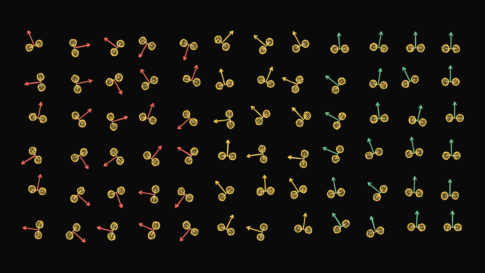
I always wondered why the word "high-temperature" in high-temperature superconductors feels like a joke. These are the copper oxide materials, the cuprates, discovered in the late 1980s, and they carry electricity with zero resistance at temperatures you can reach with liquid nitrogen instead of liquid helium. That was a huge deal, and then nothing really moved for almost forty years. We still need cryogenics, and physicists still don't agree on why cuprates superconduct in the first place.
So when a paper from Milan Allan's group at LMU Munich and Ingmar Swart's group at Utrecht landed in Science this year, I read it three times. They did something I found genuinely beautiful: they listened to the electrical crackle of current flowing into a cuprate and used it to hear electrons travelling in pairs. Their conclusion was that the pairs form at a much higher energy than anyone expected, and that the real bottleneck for superconductivity is getting those pairs to move together.
That conclusion is the part I couldn't stop thinking about, because the experiment can hear pairs but it cannot hear whether they are moving together. So I did what any normal person would do on a weeknight. I broke the problem down to first principles, found a question nobody had simulated, pre-registered my hypotheses, got two of them killed by an adversarial reviewer before writing any code, ran 3,328 Monte Carlo simulations, and was wrong about one of the things I was most confident about. This is that story.
the missing electrons
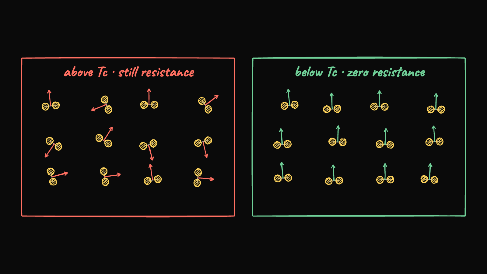
Every cuprate has a weird regime called the pseudogap. As you cool the material toward its superconducting temperature, Tc, electrons start going missing. Spectroscopy finds far fewer of them at the energies where they should be, as if a gap has opened in the electronic spectrum before superconductivity has even started.
There have been two big camps for decades. One camp says the electrons are frozen into some pattern, like a charge density wave, and superconductivity is a separate thing that happens later. The other camp says the electrons are missing because they have already paired up into Cooper pairs, the same pairs that carry supercurrent, and they are just waiting around for something else before the material actually superconducts. Basically, a waiting room for pairs.
Settling this has been brutal because every instrument sees something, and nothing is conclusive. You need a way to directly detect pairs, and that's where the noise comes in.
listening to the rain
Imagine rain on a tin roof. If every drop suddenly became twice as heavy but half as frequent, the average amount of water hitting the roof is the same, but the sound gets louder and more crackly. Each impact is bigger.
Current is the same. It is made of discrete charges arriving at random, and that randomness produces a tiny fluctuation called shot noise. If you measure the noise S and the average current I, you can read off the charge per event, because S = 2qI. Single electrons give q = 1e. Pairs give q = 2e.
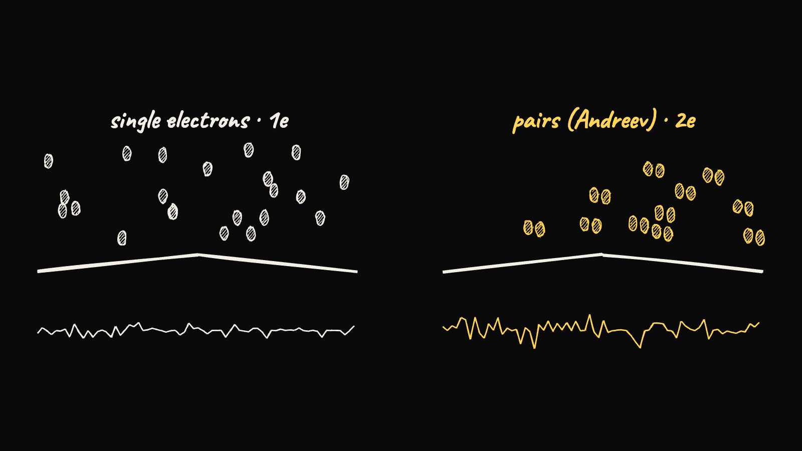
The team used a scanning tunnelling microscope, a needle so sharp it ends in roughly one atom, and passed current between the tip and a crystal of the cuprate BSCCO at a few kelvin. By changing the voltage they could pick which electron energy they were listening to, a bit like turning a radio dial. The tip is a normal metal, so a pair can't jump into it whole. Instead an electron goes in and a hole bounces back, a process called Andreev reflection, and the net effect is 2e transferred.
In a cuprate the signal is tiny. The superconducting gap has nodes, directions where single electrons keep flowing freely, so only a few percent of the current is pairs and q sits around 1.03 to 1.09e instead of 2e. It took the students years of electronics work to hear it. And what they heard was clean: the noise steps up exactly at the local pseudogap energy, at every spot they measured, with a slope of one across positions and across samples with different chemistry. In a magnetic field the extra noise fades back toward 1e. Pairing lives at the pseudogap energy, up to around 70 meV.
the blind spot
This is what broke my brain a little. Shot noise measures the size of the local pair amplitude, mathematically something like |F|², the squared magnitude of what physicists call the anomalous Green function. It does not measure the pair's quantum phase at all. It can't, because the noise is gauge invariant.
Think of each region of the material as a clock. The length of the hand is how strongly electrons are paired. The direction the hand points is the quantum phase. Superconductivity needs every clock in the sample pointing the same way, because that is what lets pairs move together as one coherent fluid with zero resistance. Noise reads the length of the hand and nothing else.
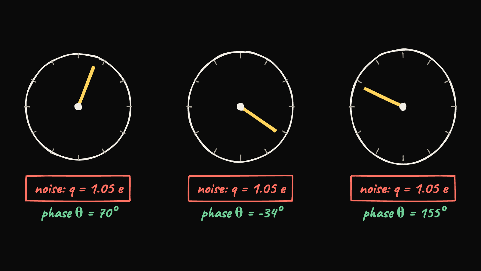
So the paper's big claim, that Tc in cuprates is limited by phase coherence rather than pairing, is a very reasonable inference, but it is an inference. The authors are honest about this. They couldn't measure above Tc yet, and Swart says he wants a separate instrument for coherence. Reading that, the question I couldn't let go of was simple. If you had the pairing map they measured, could you predict where coherence lives and what Tc is? Or is coherence something you can only get by actually simulating all the phase fluctuations?
first principles before code
I did not want to vibe this. I've seen too many simulations that are basically a pretty picture of the author's assumptions. So before any code I broke the system down into its actual parts: the pair amplitude map (measured, nanometre patches between roughly 20 and 75 meV), the local temperature where pairing dies (also measured, by Gomes and colleagues in 2007, who found 2Δ/k_B T_p ≈ 7.9), the phase stiffness (how much energy it costs to twist the phase, which is not directly measured at the nanometre scale), and the probe.
Then I generated eight candidate questions and ran a literature check on them. Nobody had fed a realistic cuprate gap map into a phase-fluctuation simulation to separate where pairs exist from where they are coherent, and none of the eight papers citing the Science result had done it either. That gap was the project.
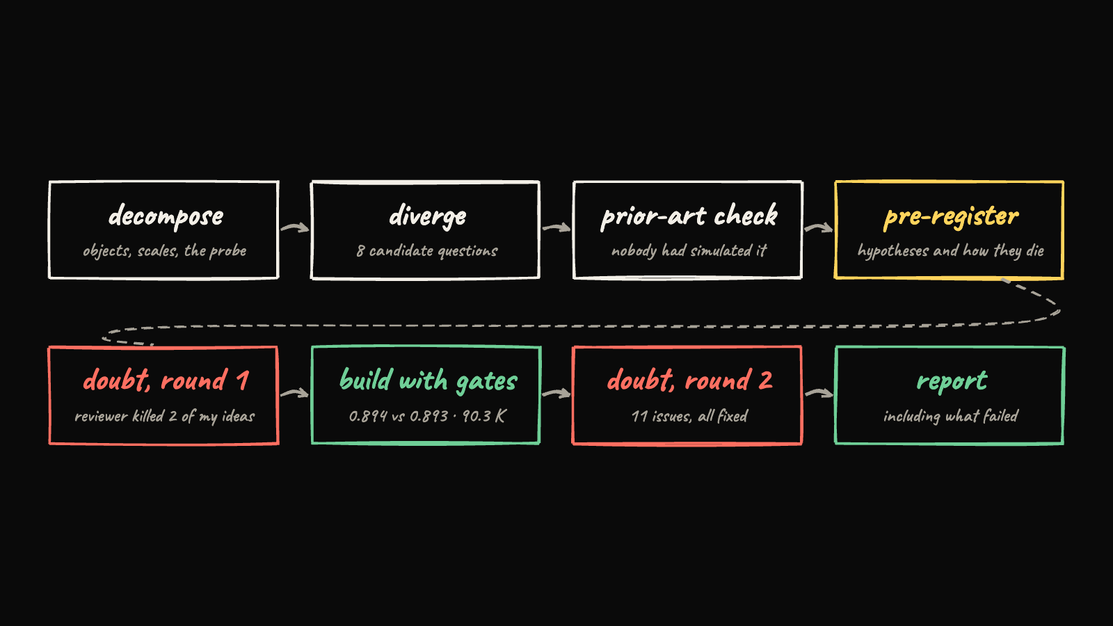
I wrote down my hypotheses, and exactly how each one would die, before running anything. Then I gave the plan to a fresh reviewer with one instruction, find what's wrong, and it found nine problems. Two of my hypotheses were rigged by construction. One was guaranteed true by the conductance law I had chosen, and another was guaranteed true because the measured pairing temperatures sit above Tc anyway. Both went in the bin. My model of the material as a grid of 1 nm tunnel junctions was replaced with a proper continuum stiffness. I'd love to say I enjoyed that review, but it was the most useful thing in the whole project.
what I actually built
The pipeline is simple to say. Generate a gap map with the same statistics as real BSCCO. Turn each patch's gap into a local pairing temperature. Turn that into a local phase stiffness using Homes' law, the empirical rule that superfluid stiffness tracks normal-state conductivity times the gap. Then simulate the phase of one copper-oxide plane with a classical XY model, which is the cleanest possible model where every site is perfectly paired and the only question is whether the phases line up.
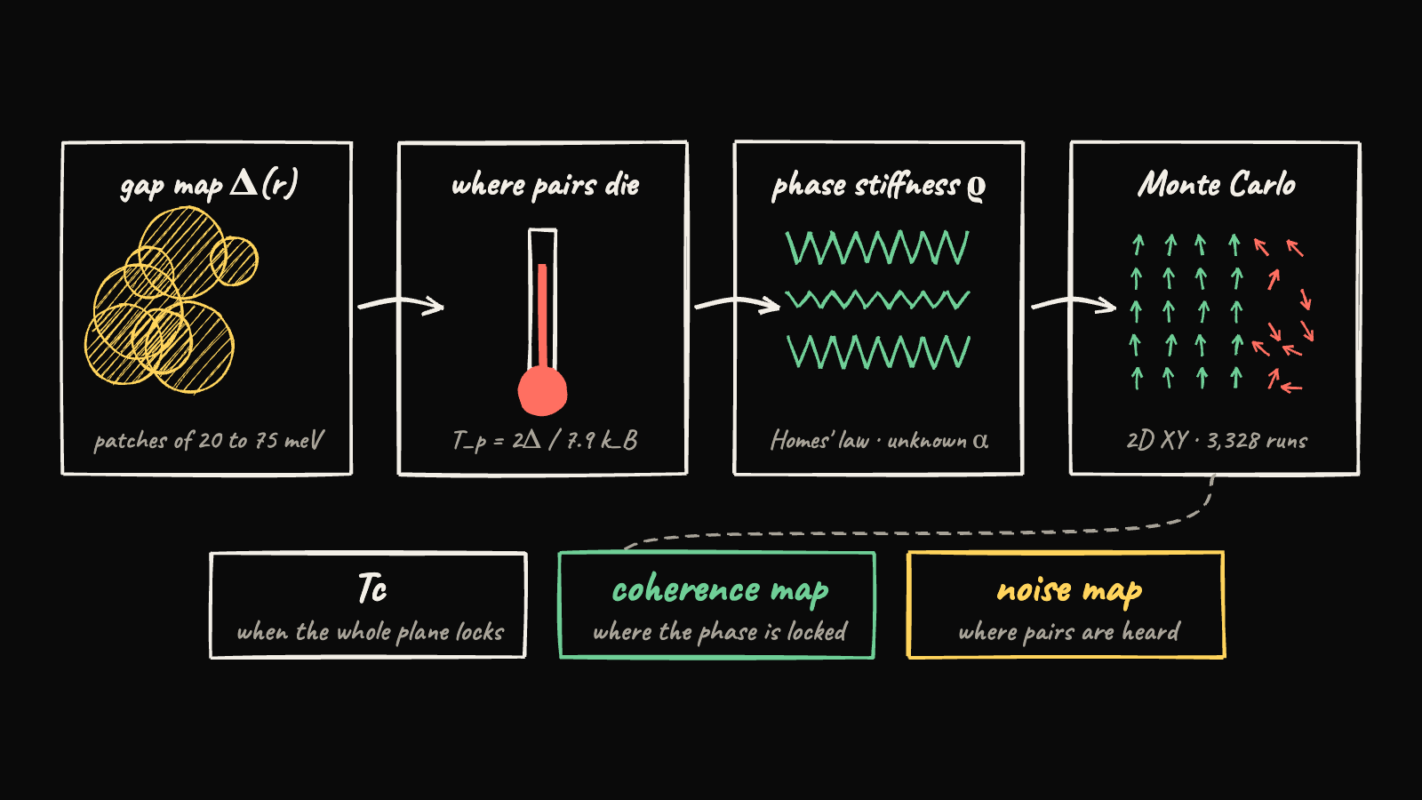
There's one honest unknown, and it ended up being the most interesting knob. Nobody knows how the local normal conductance varies with the local gap at the nanometre scale. Maybe big-gap regions conduct just as well, maybe they conduct worse. I called that exponent α and made every claim survive α = 0, 1 and 2.
Before trusting any number I made the simulator pass known physics. On a plain uniform XY model it reproduced the textbook transition temperature, 0.894 against the exact 0.893. The homogeneous BSCCO plane came out at 90.3 K against its 90 K calibration, and the first and second halves of every run agreed to 0.7 percent. Then I ran 13 disorder classes, three system sizes and eight random maps each.
The interactive below is a stripped-down version of the same simulation running in your browser. Move the temperature and watch two things separate. The pairing map barely changes, because most regions stay paired well above Tc. The phase field goes from orderly to chaotic, with vortices popping up, and that is the transition.
Tc is not an average and not a weakest link
My first pre-registered hypothesis was that you could predict Tc from the static stiffness map, without simulating anything, if you average it the right way. The two obvious guesses are the plain average (every road in a city counts equally) and the harmonic mean (traffic is set by the worst road). The less obvious one is an effective-medium average, an old trick from the physics of random resistor networks that treats the whole network as one effective material.
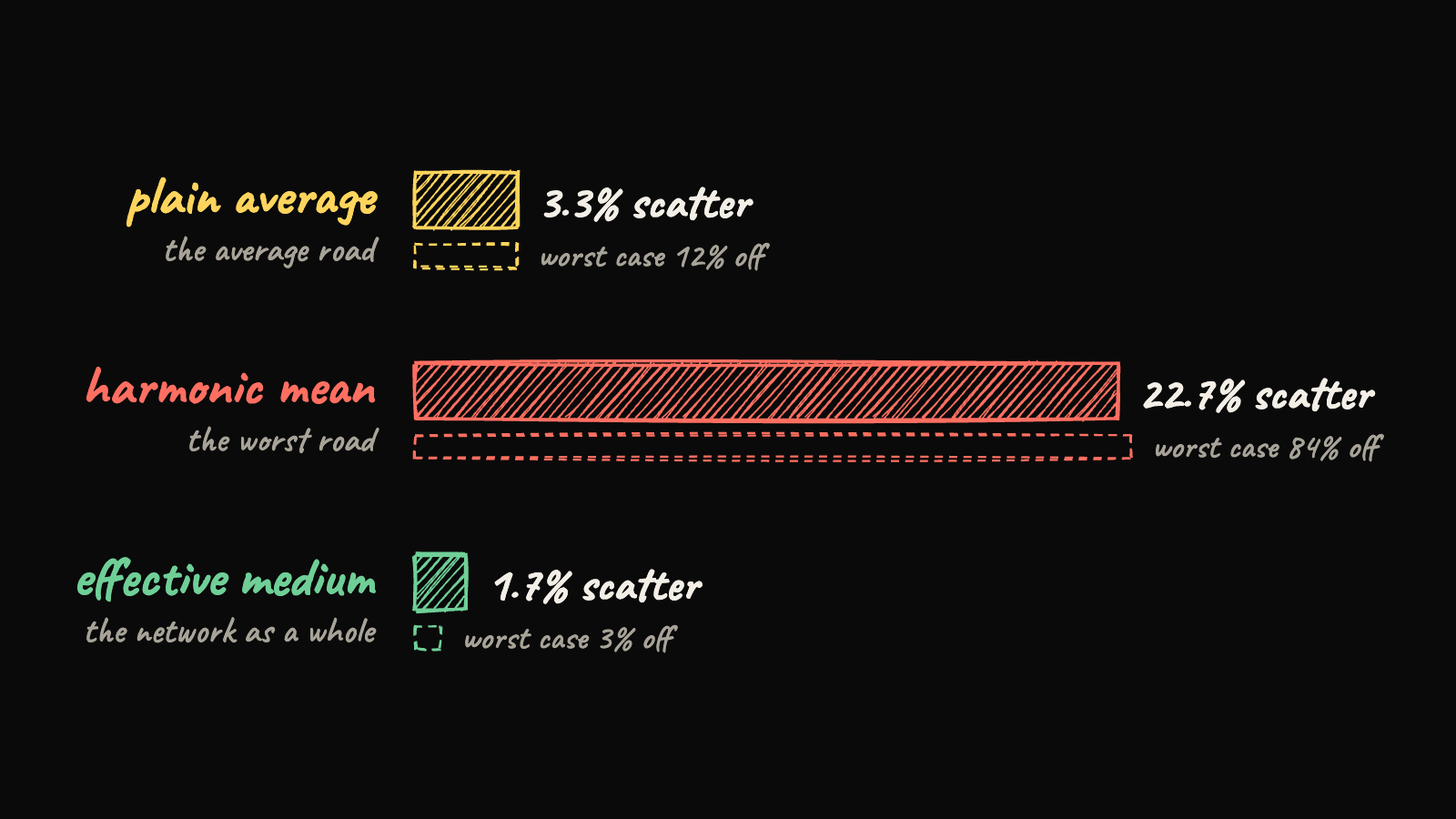
The effective medium won by a lot. Across 104 random maps it predicted the Monte Carlo Tc with 1.7 percent scatter and a mean ratio of 1.003, with nothing fitted to the heterogeneous results. The plain average had 3.3 percent scatter but was off by up to 12 percent on the most disordered maps, and the weakest-link guess was a disaster at 23 percent. It also held at every system size. The stricter hierarchical bootstrap was borderline (one-sided p ≈ 0.05), so I'll call it supported, not proven.
The other number that came out of this is how much heterogeneity costs you. At the same average gap, a patchier map lowers Tc by 2 to 6 percent at the mildest disorder, 7 to 11 percent at the realistic level, and 14 to 18 percent at the strongest. That matters for anyone dreaming about tuning cuprates by chemistry, because a uniform material at the same average pairing strength just does better.
I was wrong about where coherence lives
My second hypothesis was the one I was most confident about. I thought coherence would live along the "backbone" of the network, the paths that carry the supercurrent, like the main roads in a city. So I computed that backbone from the static map and checked whether it predicted where the simulated phase was locked.
It didn't. The correlation was 0.03 to 0.14, basically noise, so the hypothesis was falsified by the exact criterion I wrote down in advance. The local stiffness of each patch did much better, 0.67 to 0.92 depending on α.
What actually nailed it was something older and simpler, spin-wave theory. If you pretend the phase only wiggles gently, with no vortices at all, you can compute from the stiffness map alone how much each patch's phase fluctuates. That got 97 percent of the way to the best correlation the noise in my simulation even allows. So vortices are what destroy superconductivity at Tc, but the spatial pattern of where coherence survives is basically set by gentle wiggles on the stiffness map. I did not expect that, and I'm glad I wrote the hypothesis down before running, because otherwise I'd have been tempted to quietly redefine "backbone" until it worked.
pairs survive, coherence doesn't
This is the picture I wanted from the start. Below is the real simulation output as a 3D volume, with the map as the floor and temperature going up. Red is where a noise-STM would still detect pairs. Blue is where the phase is locked.
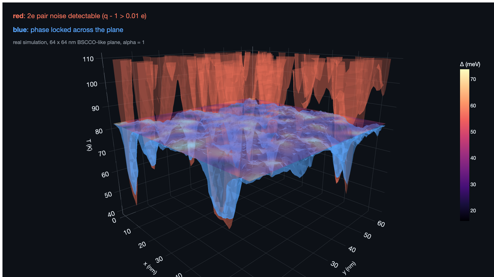
At Tc about 95 percent of the plane would still show detectable pair noise, while coherence collapses within a few kelvin. The red chimneys keep going up to 110 K over the strong patches. If you only had a noise microscope, the superconducting transition would be nearly invisible.
I want to be careful about one number here. The fraction of the plane that is "paired but not coherent" swings anywhere from about 1 to 97 percent depending on where you draw the thresholds, so I don't trust it as a headline. What is robust is a correlation between maps, which leads to the part I'm most excited about.
a prediction someone can actually test
Take one patch of BSCCO. Map its gap with a normal STM, and map its coherence with a Josephson STM, which uses a superconducting tip and is sensitive to the phase. Then just correlate the two maps slightly below Tc.
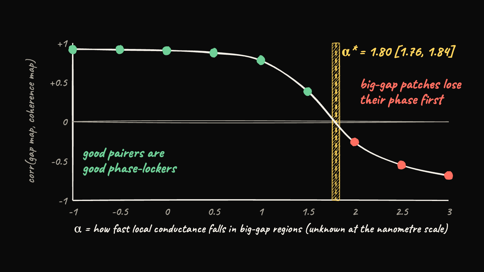
In the simulation that correlation is +0.88 if big-gap regions conduct normally (α = 0), +0.77 at α = 1, and drops to +0.09 at α = 2. It changes sign at α ≈ 1.80, with a confidence interval of 1.76 to 1.84. A positive correlation means good pairers are also good phase-lockers. A negative one means the big-gap regions are poor conductors that lose their phase first. Either way, two existing microscopes pointed at the same 64 nm patch would measure a property of the material that no single instrument can see right now.
One honest caveat. In my model the noise map and the gap map carry the same information about α, because the noise rises steadily with the gap, so you don't strictly need noise for this. What noise adds is the proof that the gap you're mapping is a pairing gap, which is exactly what the Science paper established.
for the nerds who want the receipts
Everything below is optional. The full notebook with every cell, figure and number is public on Kaggle.
The probe. For Poisson tunnelling events of charge q, the current noise is
and if a fraction f of the current is carried by 2e events, the effective charge is q/e = 1 + f. Andreev reflection scales as τ² in the barrier transparency τ, while single-quasiparticle tunnelling scales as τ, which is why d-wave nodes swamp the pair signal. I modelled the tip with the d-wave Blonder–Tinkham–Klapwijk formalism with complex-energy (Dynes) broadening and Fermi smearing.
The input map. A periodic Gaussian random field Δ_i with mean 45 meV, standard deviation 5, 9 or 13 meV, and correlation length 2.5 nm (or uncorrelated as a control). The local amplitude follows a BCS shape and vanishes at
from the Gomes et al. gap maps through Tc.
The stiffness. Dirty-limit (Homes' law) local stiffness with the unknown gap–conductance exponent α,
with bonds given by the harmonic face average ρ_ij = 2ρ_iρ_j/(ρ_i + ρ_j), which is the flux-conserving discretisation of ∇·(ρ∇θ). ρ_0 is fixed once so the homogeneous plane has Tc = 90 K.
The simulation. A classical 2D XY model,
sampled with Metropolis plus Wolff cluster updates in numba, on L = 32, 48 and 64 lattices. Tc comes from where the helicity modulus Υ crosses the Berezinskii–Kosterlitz–Thouless line 2T/π, extrapolated in 1/ln²L.
for each disorder class, map, size L, temperature T:
    rho_ij = bonds(stiffness(gap_map, T, alpha))
    equilibrate(theta, rho_ij, T)             # Metropolis + Wolff
    measure helicity modulus and far-field phase correlation C_i
Tc = T where helicity(T) crosses 2T/pi       # then 1/ln(L)^2 extrapolation
The estimators. Each solves T = 0.893 ρ_est(T), exact for the uniform plane. The effective medium value ρ_m solves the Kirkpatrick condition on the square lattice,
Coherence and spin waves. The gauge-invariant coherence of site i is C_i = ⟨cos(θ_i − θ_j)⟩ averaged over sites more than L/4 away. The spin-wave prediction uses the pseudo-inverse G of the stiffness Laplacian, with phase-difference variance T(G_ii + G_jj − 2G_ij).
What it is not. It is one classical copper-oxide plane with synthetic but statistics-matched maps. Interlayer coupling (about 10⁻⁴ of the in-plane value in BSCCO) is only estimated to shift every Tc up by a few percent. Quantum phase fluctuations and feedback between amplitude and phase are ignored, and the Josephson STM signal is a proxy. Every pre-registered hypothesis, deviation and both adversarial reviews are written into the notebook, including my first "local order" model that faked the result because a density-of-states peak inflated the pair signal.
my honest take
I came in thinking this was a story about pairs. It's really a story about phase, and about how much of the phase story you can get from a static map if you average it the way physics wants instead of the way spreadsheets want. The effective-medium result made me oddly happy, because it means a nanometre gap map plus one unknown exponent gets you most of the way to Tc, and that unknown exponent is something two existing microscopes could pin down next month.
Allan said in an interview that he has more hope in chemistry and trial and error than in pure physics for pushing Tc higher. After this, I think the two meet in the middle. Make the pairing landscape smoother, and make sure the strong pairers are also good conductors, because in this model pairing was never the bottleneck. 🫡